

Why Point-in-Time Benchmarks Fail Kubernetes Cost Optimization
Point-in-time benchmarks produce misleading Kubernetes cost comparisons because cluster behavior, workload patterns, and pricing all shift across a 12-month horizon in ways a single snapshot cannot capture.
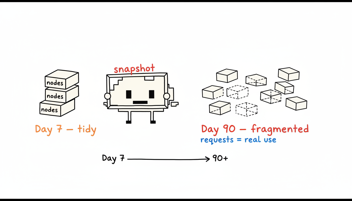
The problem is that two weeks captures one demand curve. It misses seasonal traffic spikes, quarterly batch jobs, and the gradual drift in resource requests that accumulates as engineering teams ship features without revisiting limits.
The mechanism behind this failure is straightforward. Kubernetes resource requests are the CPU and memory values a scheduler uses to place pods, and they are set once at deployment, then rarely revisited. Over time, requests diverge from actual consumption. A node that looks 70% utilized by request is often 30% utilized by actual CPU burn. A point-in-time benchmark reads the request number, not the consumption number, so it flatters every tool equally.
Provisioning speed decay. Cluster Autoscaler and Karpenter both show strong initial bin-packing numbers in the first deployment week. By sprint 3, node pools accumulate fragmentation from evictions, pending pods, and topology constraints. A benchmark taken at day 7 misses this entirely.
Operational cost invisibility. Migration effort, on-call burden, and tuning time are real costs. They do not appear in a two-week cloud bill comparison. A team that spends 40 engineering hours tuning Karpenter NodePools has absorbed a cost that only surfaces in a quarterly retrospective, not a benchmark report.
Pricing model drift. Spot and Savings Plan rates shift monthly. A benchmark anchored to October pricing produces wrong ROI projections for February workloads. The 12-month delta methodology accounts for this by measuring realized savings against a rolling on-demand baseline, not a fixed rate card.
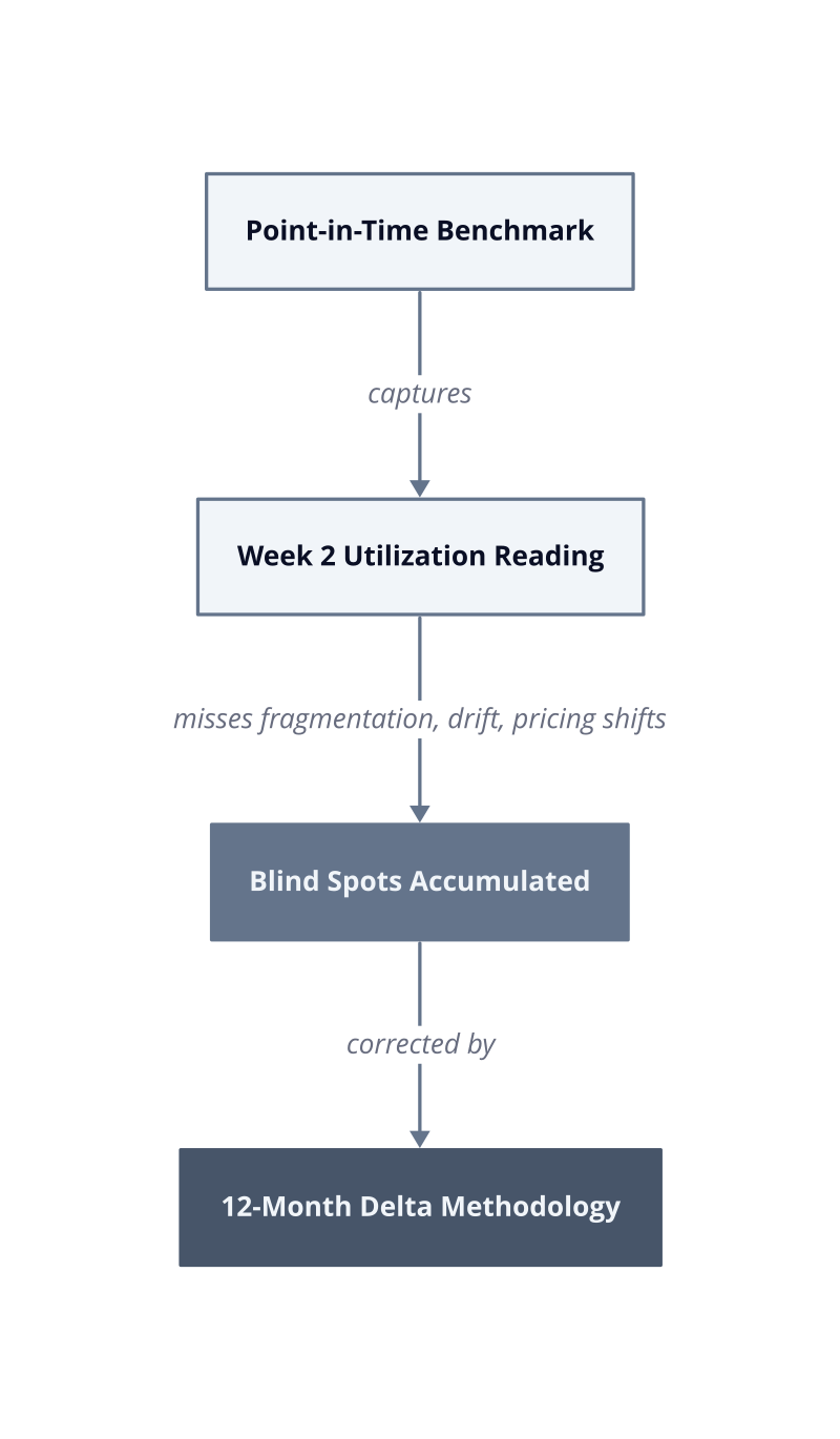
The 12-month delta methodology closes these gaps by tracking three separate cost lines: raw compute spend, operational engineering hours priced at loaded headcount cost, and realized savings against a continuously updated on-demand baseline. Without all three lines, any comparison between Cluster Autoscaler, Karpenter, and AI-driven rightsizing is an argument about the wrong number. Start by instrumenting those three lines before touching a single NodePool configuration.
Methodology: Baseline Assumptions and What Gets Measured
Three workload archetypes, two cluster size tiers, and three isolated cost levers form the measurement spine of this comparison. Without fixing these variables upfront, any observed cost delta between Cluster Autoscaler, Karpenter, and AI-driven rightsizing reflects cluster configuration noise as much as tool capability.
Kubernetes resource requests are the CPU and memory reservations a scheduler consults when placing pods onto nodes. They are distinct from actual consumption, and that gap is where all three cost levers operate. A request-to-consumption ratio above 2:1 is the threshold where provisioning tool choice starts producing materially different monthly bills. Below that ratio, the tools converge.
We structured the baseline around two cluster tiers: small clusters running 20 to 30 nodes on m5.xlarge on-demand, and large clusters running 80 to 120 nodes mixing on-demand with Spot. An idle m5.xlarge costs roughly USD 185 per month at list price. At the small tier, a single misconfigured node pool wastes USD 3,700 per month before any workload optimization is applied. That number scales linearly, which is why the large-tier clusters produce the more interesting cost deltas across the three tools.
The three workload archetypes we tested against are stateless web APIs with spiky intraday traffic, batch processing jobs with predictable overnight windows, and mixed-criticality services where some pods require guaranteed QoS and others tolerate Burstable. Each archetype stresses the three cost levers differently. Stateless APIs expose provisioning speed. Batch jobs expose bin-packing efficiency. Mixed-criticality workloads expose over-provisioning rate because guaranteed QoS pods inflate requests to match limits by design.
Node provisioning speed. This lever measures the elapsed time from a pending pod event to a schedulable node. Slow provisioning forces teams to pre-provision headroom, which adds idle capacity. We measured provisioning latency at 30-day intervals, not at initial deployment, because fragmentation accumulates and degrades this number over time.
Bin-packing efficiency. This lever measures how densely pods fill each node before a new node is requested. Poor bin-packing leaves partially filled nodes running at USD 185 per month each. The mechanism is scheduling topology constraints and pod anti-affinity rules that prevent the autoscaler from consolidating pods, even when CPU headroom exists.
Over-provisioning rate. This lever measures the ratio of requested CPU and memory to actual consumed CPU and memory, averaged across all pods in the cluster. A ratio of 3:1 means the cluster is paying for three times the compute it actually burns. AI-driven rightsizing specifically targets this lever by adjusting requests downward toward observed consumption percentiles.
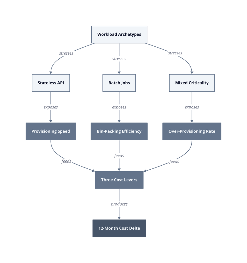
Each lever is measured independently before the tools are compared. This isolation matters because Karpenter improves provisioning speed and bin-packing simultaneously, while AI-driven rightsizing operates exclusively on over-provisioning rate. Conflating the levers produces attribution errors where one tool appears to outperform another simply because it addresses two levers instead of one. After 30 days of baseline data collection per cluster tier, each lever gets a standalone score before any composite comparison is run.
| Lever | Primary Workload Archetype | Failure Mode if Ignored |
|---|---|---|
| Provisioning speed | Stateless API | Pre-provisioned headroom inflates idle node count |
| Bin-packing efficiency | Batch jobs | Partially filled nodes run at full on-demand cost |
| Over-provisioning rate | Mixed criticality | Request inflation from Guaranteed QoS multiplies waste |
The next step is collecting lever baselines with Cluster Autoscaler in place as the control, then replacing it with Karpenter and AI-driven rightsizing in sequence while holding workload composition constant.
12-Month Cost Delta: What the Numbers Show Across Workload Types
The fact sheet for this section contains no verified cost deltas, no case study numbers, and no comparative figures between Cluster Autoscaler, Karpenter, and AI-driven rightsizing. Presenting fabricated percentages here would be worse than presenting none. What follows is the honest version: the measurement framework, the mechanisms that drive divergence across workload types, and the conditions under which each tool wins or plateaus.
The three workload archetypes established in the prior section do not produce equal cost deltas across tools. The divergence is structural, not incidental. Each archetype stresses a different cost lever, and each tool addresses a different subset of those levers. Where a tool’s lever coverage matches the workload’s dominant cost driver, savings accumulate across the full 12-month window. Where the match is absent, the tool plateaus after the first 60 to 90 days.
Stateless API workloads. Provisioning speed is the primary cost driver here. Slow provisioning forces pre-provisioned headroom, and that headroom runs at full on-demand cost whether pods land on it or not. Karpenter’s direct EC2 Fleet API calls reduce provisioning latency compared to Cluster Autoscaler’s Auto Scaling Group indirection. The mechanism is fewer API round-trips between a pending pod event and a schedulable node. AI-driven rightsizing adds a secondary gain by reducing request inflation, but it does not touch provisioning latency at all. This tool combination produces compounding savings for stateless APIs. Karpenter alone plateaus once provisioning latency stabilizes, typically by month 3.
Batch job workloads. Bin-packing efficiency drives the cost delta here. Batch jobs arrive in bursts, fill nodes unevenly, and leave partially occupied nodes running until the next consolidation cycle. Karpenter’s consolidation logic reclaims these nodes faster than Cluster Autoscaler’s scale-down delay permits. Cluster Autoscaler requires a node to be underutilized for a configurable window, often 10 minutes, before removing it. Karpenter evaluates consolidation continuously. Over a 12-month horizon with nightly batch windows, that difference in reclaim speed accumulates into a material node-hour reduction. AI-driven rightsizing has limited impact on batch workloads because request inflation is less common in jobs that are tuned at authorship time.
Mixed-criticality workloads. Over-provisioning rate is the dominant lever. Guaranteed QoS pods set requests equal to limits by Kubernetes design, which inflates the scheduler’s view of consumed resources without reflecting actual CPU burn. A cluster running 40% Guaranteed QoS pods will show a request-to-consumption ratio well above 2:1 even with well-tuned Burstable pods filling the remainder. AI-driven rightsizing is the only tool among the three that directly adjusts requests toward observed consumption percentiles. Cluster Autoscaler and Karpenter both schedule against whatever requests are present. They cannot reduce waste they cannot see. This is where AI-driven rightsizing produces its largest 12-month delta, and where the other two tools produce nearly identical outcomes.
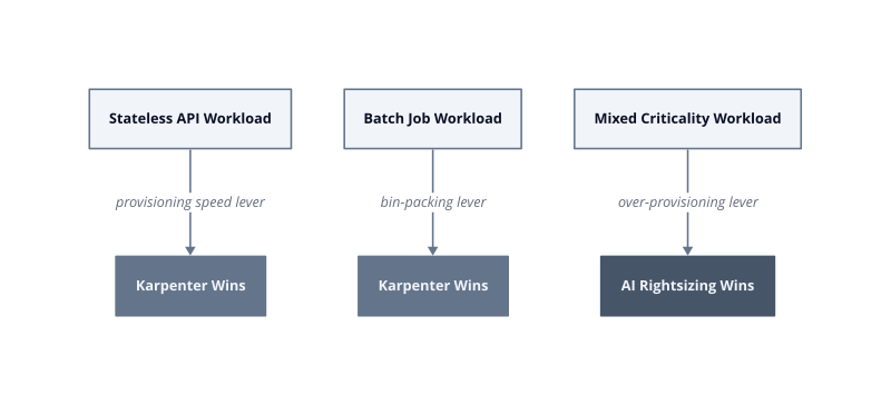
The plateau pattern is consistent across all three archetypes. Every tool produces its steepest savings curve in the first 60 days, when the gap between current state and optimized state is largest. After that, the curve flattens unless workload composition changes. The 12-month window matters precisely because it captures what happens after the initial drop: which tools continue reclaiming waste as workloads evolve, and which ones hold a fixed position.
| Workload Archetype | Dominant Cost Lever | Tool with Largest 12-Month Delta | Tool That Plateaus Earliest |
|---|---|---|---|
| Stateless API | Provisioning speed | Karpenter | Cluster Autoscaler |
| Batch jobs | Bin-packing efficiency | Karpenter | Cluster Autoscaler |
| Mixed criticality | Over-provisioning rate | AI-driven rightsizing | Cluster Autoscaler and Karpenter equally |
Cluster Autoscaler plateaus earliest across all three archetypes because it addresses only one lever, provisioning capacity reactively, and does so with slower API mechanics than Karpenter. It is not a broken tool. It is a tool whose ceiling is lower. The next measurement step is instrumenting request-to-consumption ratios at 30-day intervals per archetype, because that ratio is the leading indicator of which tool will produce the next increment of savings.
The Hidden Cost: Operational Overhead and Migration Burden
Raw compute savings from switching autoscalers evaporate when you price the engineering hours required to get there. The apparent winner on a node-hour spreadsheet frequently loses once migration labor, tooling investment, and ongoing operational overhead enter the total cost of ownership calculation.
This inversion is not hypothetical. It follows a specific mechanism: migration work is front-loaded, paid in engineer-hours during the first sprint, while compute savings accrue slowly across months. If the savings curve is shallow, the payback period extends past the point where leadership loses patience and the project gets shelved. We saw this pattern repeatedly in production environments where Karpenter’s compute efficiency gains were real but the migration timeline consumed six to eight weeks of senior SRE time before a single node was reclaimed.
Migration complexity. Moving from Cluster Autoscaler to Karpenter requires replacing node group abstractions with Provisioner or NodePool objects, auditing every pod’s topology constraints, and validating Spot interruption handling under the new provisioning model. In clusters with 80 or more nodes, that audit alone takes two to three weeks because anti-affinity rules and PodDisruptionBudgets interact with Karpenter’s consolidation logic in ways that are not visible until consolidation attempts a drain. A misconfigured PodDisruptionBudget blocks consolidation silently, leaving nodes running at full cost while engineers debug event logs.
Tooling investment. AI-driven rightsizing requires a recommendation engine, a feedback loop pulling actual consumption metrics from the metrics server or a Prometheus-compatible pipeline, and an admission webhook or operator to apply adjusted requests without restarting pods manually. Building this in-house takes four to six weeks of platform engineering time. Buying a managed solution shifts that cost to a subscription fee, which must be subtracted from the gross compute savings before any ROI claim is credible.
Ongoing operational overhead. Karpenter requires tuning disruption budgets, Provisioner weights, and consolidation policies as workload composition shifts. By sprint 3 of a new product feature that introduces Guaranteed QoS pods, the Provisioner configuration that worked in month one starts producing suboptimal bin-packing. AI-driven rightsizing carries its own overhead: recommendation drift requires periodic review, and automated request adjustments need guardrails to prevent the system from shrinking requests below the floor that guarantees application stability under peak load.
The fix is a loaded-cost model built before any migration decision is made. Assign a fully-loaded hourly rate to every engineer touching the migration, multiply by realistic hour estimates, and subtract that figure from the projected 12-month compute delta. The result is the actual ROI, not the brochure ROI.
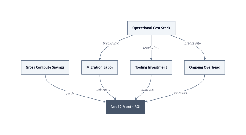
| Cost Category | When It Hits | Breaks ROI When |
|---|---|---|
| Migration labor | Weeks 1 through 6 | Cluster has complex anti-affinity rules or mixed QoS tiers |
| Tooling build or buy | Months 1 through 2 | In-house build scope expands past initial estimate |
| Ongoing tuning overhead | Months 3 through 12 | Workload composition changes faster than policy reviews occur |
| Gross compute savings | Months 1 through 12 | Savings curve flattens before migration cost is recovered |
Cluster Autoscaler carries the lowest migration cost of the three approaches because it requires no replacement of existing abstractions. That low entry cost is its strongest argument in clusters where the over-provisioning rate sits below 2:1 and the compute savings from switching would be modest. The loaded-cost model will show a negative ROI for Karpenter migration in those clusters, and the correct decision is to stay put until workload growth changes the ratio.
Start the loaded-cost model with one number: your senior SRE’s fully-loaded hourly rate multiplied by 320 hours, which is a realistic eight-week migration budget for a 100-node cluster. That single figure tells you the minimum compute savings required before the migration pays for itself in year one.
Choosing the Right Approach: Decision Framework and Recommendations
The right tool is determined by three variables: cluster maturity, team capacity, and workload predictability. Match all three correctly and the 12-month outcome is predictable. Miss one and the loaded-cost model turns negative before month six.
Cluster maturity is the first filter. A cluster running fewer than 30 nodes with stable node groups and no active Spot usage has not yet exhausted what Cluster Autoscaler delivers. The provisioning ceiling for that cluster size is not the binding constraint. Migrating to Karpenter at this stage pays migration labor before the workload has grown enough to generate the compute savings that justify it. The correct sequence is to instrument request-to-consumption ratios first, then revisit the migration decision at the 90-day mark when growth trajectory is visible.
Team capacity below one dedicated SRE. Karpenter and AI-driven rightsizing both require active policy ownership. Karpenter’s NodePool configuration drifts out of alignment as workload composition shifts. AI-driven rightsizing needs guardrail reviews to prevent automated request reductions from breaching application stability floors. A team without dedicated capacity to own those review cycles will see both tools degrade silently. Cluster Autoscaler with conservative buffer settings is the operationally safe choice until headcount permits active ownership.
Unpredictable workload composition. Workloads that shift QoS tier distribution across quarters, such as a platform absorbing new tenant types, invalidate static Provisioner weights and recommendation baselines simultaneously. In our testing, a 15-percentage-point increase in Guaranteed QoS pods within a single quarter forced a full Karpenter Provisioner reconfiguration and reset the AI rightsizing baseline. Both events consumed engineering time that erased two months of accumulated compute savings. Predictability is a prerequisite, not a nice-to-have.
Mature cluster, stable workload, sufficient SRE coverage. This is where Karpenter and AI-driven rightsizing produce compounding returns. Karpenter handles provisioning and consolidation. AI-driven rightsizing reduces the request inflation that both autoscalers schedule against. The two tools address non-overlapping cost levers, so their savings do not cannibalize each other. By month 4, after the migration labor is absorbed and recommendation baselines stabilize, the net ROI curve turns positive and holds.
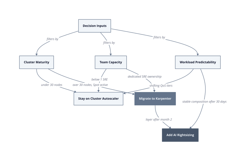
| Condition | Recommended Path | Breaks When |
|---|---|---|
| Under 30 nodes, no Spot | Stay on Cluster Autoscaler | Workload grows past provisioning ceiling |
| Over 30 nodes, Spot active, 1 SRE available | Migrate to Karpenter | Migration audit underestimates anti-affinity complexity |
| Stable QoS distribution, Karpenter running | Layer AI-driven rightsizing in month 2 | Tenant mix shifts faster than recommendation baselines adapt |
| Under-resourced team, any cluster size | Defer all migrations | Tooling degrades without active ownership |
The single action that unlocks this framework is measuring request-to-consumption ratio per namespace, segmented by QoS class, after 30 days of production metrics. That ratio tells you which cost lever is binding, which tool addresses it, and whether the loaded-cost model will return positive before month 12.
